Bayesian inference

Bayesian inference is a method of statistical inference in which some kind of evidence or observations are used to calculate the probability that a hypothesis may be true, or else to update its previously-calculated probability. The term "Bayesian" comes from its use of the Bayes' theorem in the calculation process. Bayes' theorem was deduced in several special cases by Thomas Bayes, and then it was extended to the general theorem by other researchers.^[1]

Evidence and changing beliefs

The primary foundation of Bayesian inference is the Bayesian interpretation of probability, which is distinct from other interpretations of probability (see: probability interpretations) in that it permits the attribution of probabilities to the truth and falsehood of events that are not random, but rather the truth or untruth of which is simply unknown.

Bayesian inference uses aspects of the scientific method, the method which involves collecting evidence that will be either consistent or inconsistent with a given hypothesis. As the evidence accumulates, the degree of confidence in a hypothesis ought to change. With enough evidence, the degree of confidence should become either very high or very low. Thus, proponents of Bayesian inference say that it can be used to discriminate between conflicting hypotheses: hypotheses with very high support should be accepted as true, and those with very low support should be rejected as false. However, detractors say that this inference method might be biased due to initial notions that one holds before any evidence is ever collected. (This is a form of inductive bias.)

Bayesian inference uses a numerical estimate of the degree of confidence in a hypothesis before any evidence has been observed, and then it calculates a numerical estimate of the degree of confidence in the hypothesis after a set of evidence has been observed. (This process is repeated whenever additional evidence is obtained.) Bayesian inference usually relies on degrees of belief, or subjective probabilities, in the induction process, and it does not necessarily claim to provide an objective method of induction. Nonetheless, some Bayesian statisticians think that probabilities can have an objective value, and therefore Bayesian inference can provide an objective method of induction. See scientific method.

Bayes' theorem modifies probabilities, given new pieces of evidence, in the following way:

$P(H|E) = \frac{P(E|H)\;P(H)}{P(E)}$

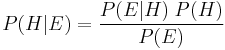
where

$H$ represents a specific hypothesis, which may or may not be some null hypothesis.
$E$ represents the evidence that has been observed.
$P(H)$ is called the prior probability of $H$ that was inferred before new evidence became available.
$P(E|H)$ is called the conditional probability of seeing the evidence $E$ if the hypothesis $H$ happens to be true. It is also called a likelihood function when it is considered as a function of $H$ for fixed $E$ .
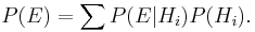
$P(E)$ is called the marginal probability of $E$ : the a priori probability of witnessing the new evidence $E$ under all possible hypotheses. It can be calculated as the sum of the product of all probabilities of any complete set of mutually exclusive hypotheses and corresponding conditional probabilities:

$P(E) = \sum P(E|H_i)P(H_i).$

$P(H|E)$ is called the posterior probability of $H$ given $E$ and is the new estimate of the probability that the hypothesis $H$ is true, taking the evidence $E$ into account.

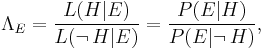
The factor 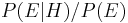$P(E|H) / P(E)$ represents the impact that the evidence has on the belief in the hypothesis. If it is likely that the evidence $E$ would be observed when the hypothesis under consideration is true, but, when no hypothesis is assumed, it is inherently unlikely that $E$ would have been the outcome of the observation, then this factor will be large. Multiplying the prior probability of the hypothesis by this factor would result in a larger posterior probability of the hypothesis given the evidence. Conversely, if it is unlikely that the evidence $E$ would be observed if the hypothesis under consideration is true, but a priori likely that $E$ would be observed, then the factor would reduce the posterior probability for $H$ . Under Bayesian inference, Bayes' theorem therefore measures how much new evidence should alter a belief in a hypothesis.

Bayesian statisticians argue that even when people have very different prior subjective probabilities, new evidence from repeated observations will tend to bring their posterior subjective probabilities closer together. However, others argue that when people hold widely different prior subjective probabilities their posterior subjective probabilities may never converge even with repeated collection of evidence. These critics argue that worldviews which are completely different initially can remain completely different over time despite a large accumulation of evidence.

Multiplying the prior probability $P(H)$ by the factor $P(E|H) / P(E)$ will never yield a probability that is greater than 1, since $P(E)$ is at least as great as $P(E \cap H)$ (where $\cap$ denotes "and"), which equals 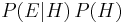$P(E|H)\,P(H)$ (see joint probability).

The probability of $E$ given $H$ , $P(E|H)$ , can be represented as a function of its second argument with its first argument held fixed. Such a function is called a likelihood function; it is a function of $H$ alone, with $E$ treated as a parameter. A ratio of two likelihood functions is called a likelihood ratio, $\Lambda$ . For example,

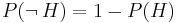
$\Lambda_E = \frac{L(H|E)}{L(\neg\,H|E)} = \frac{P(E|H)}{P(E|\neg\,H)},$

where the dependence of $\Lambda_E$ on $H$ is suppressed for simplicity (as $E$ might have been, except we will need to use that parameter below). Since $H$ and not- $H$ are mutually exclusive and span all possibilities, the sum previously given for the marginal probability reduces to

$P(E) = P(E|H)\,P(H)+P(E|\neg\,H)\,P(\neg\,H)$

As a result, we can rewrite Bayes' theorem as

$P(H|E) = \frac{P(E|H)\,P(H)}{P(E|H)\,P(H)+ P(E|\neg\,H)\,P(\neg\,H)} = \frac{\Lambda_E P(H)}{\Lambda_E P(H) +P(\neg\,H)}.$

We could then exploit the identity

$P(\neg\,H) = 1 - P(H)$

to exhibit $P(H|E)$ as a function of just $P(H)$ (and $\Lambda_E$ , which is computed directly from the evidence).

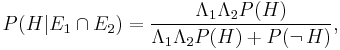
With two pieces of evidence $E_1$ and $E_2$ , that are marginally and conditionally independent of each other given the hypotheses, Bayesian inference can be applied iteratively. We could use the first piece of evidence to calculate an initial posterior probability, and then use that posterior probability as a new prior probability to calculate a second posterior probability given the second piece of evidence. Bayes' theorem applied iteratively yields

$P(H|E_1 \cap E_2) = \frac{P(E_1|H)\;P(E_2|H)\,P(H)}{P(E_1|H)\;P(E_2|H)\;P(H) + P(E_1|\neg\,H)\;P(E_2|\neg\,H)\;P(\neg\,H)}$

Using likelihood ratios, we find that

$P(H|E_1 \cap E_2) = \frac{\Lambda_1 \Lambda_2 P(H)}{\Lambda_1 \Lambda_2 P(H) + P(\neg\,H)},$

This iteration of Bayesian inference could be extended with more independent pieces of evidence.

Bayesian inference is used to calculate probabilities for decision making under uncertainty. Besides the probabilities, a loss function should be evaluated to take into account the relative impact of the alternatives.

Simple examples of Bayesian inference

Which bowl is the cookie from?

To illustrate, suppose there are two full bowls of cookies. Bowl #1 has 10 chocolate chip and 30 plain cookies, while bowl #2 has 20 of each. Our friend Fred picks a bowl at random, and then picks a cookie at random. We may assume there is no reason to believe Fred treats one bowl differently from another, likewise for the cookies. The cookie turns out to be a plain one. How probable is it that Fred picked it out of bowl #1?

Intuitively, it seems clear that the answer should be more than a half, since there are more plain cookies in bowl #1. The precise answer is given by Bayes' theorem. Let $H_1$ correspond to bowl #1, and $H_2$ to bowl #2. It is given that the bowls are identical from Fred's point of view, thus 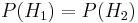$P(H_1)=P(H_2)$ , and the two must add up to 1, so both are equal to 0.5. The event $E$ is the observation of a plain cookie. From the contents of the bowls, we know that 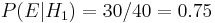$P(E|H_1) = 30/40 = 0.75$ and $P(E|H_2) = 20/40 = 0.5$ . 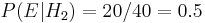Bayes' formula then yields

$\begin{align} P(H_1|E) &= \frac{P(E|H_1)\,P(H_1)}{P(E|H_1)\,P(H_1)\;+\;P(E|H_2)\,P(H_2)} \\ \\ \ & = \frac{0.75 \times 0.5}{0.75 \times 0.5 + 0.5 \times 0.5} \\ \\ \ & = 0.6 \end{align}$

Before we observed the cookie, the probability we assigned for Fred having chosen bowl #1 was the prior probability, $P(H_1)$ , which was 0.5. After observing the cookie, we must revise the probability to $P(H_1|E)$ , which is 0.6.

False positives in a medical test

False positives result when a test falsely or incorrectly reports a positive result. For example, a medical test for a disease may return a positive result indicating that patient has a disease even if the patient does not have the disease. We can use Bayes' theorem to determine the probability that a positive result is in fact a false positive. We find that if a disease is rare, then the majority of positive results may be false positives, even if the test is accurate.

Suppose that a test for a disease generates the following results:

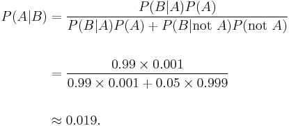
If a tested patient has the disease, the test returns a positive result 99% of the time, or with probability 0.99
If a tested patient does not have the disease, the test returns a positive result 5% of the time, or with probability 0.05.

Naively, one might think that only 5% of positive test results are false, but that is quite wrong, as we shall see.

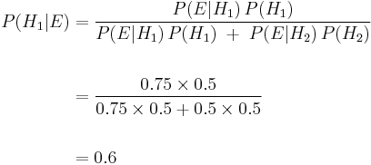
Suppose that only 0.1% of the population has that disease, so that a randomly selected patient has a 0.001 prior probability of having the disease.

We can use Bayes' theorem to calculate the probability that a positive test result is a false positive.

Let A represent the condition in which the patient has the disease, and B represent the evidence of a positive test result. Then, the probability that the patient actually has the disease given the positive test result is

$\begin{align} P(A | B) &= \frac{P(B | A) P(A)}{P(B | A)P(A) + P(B |\text{not }A)P(\text{not }A)} \\ \\ &= \frac{0.99\times 0.001}{0.99 \times 0.001 + 0.05\times 0.999} \\ ~\\ &\approx 0.019. \end{align}$

and hence the probability that a positive result is a false positive is about 1 − 0.019 = 0.98, or 98%.

Despite the apparent high accuracy of the test, the incidence of the disease is so low that the vast majority of patients who test positive do not have the disease. Nonetheless, the fraction of patients who test positive who do have the disease (0.019) is 19 times the fraction of people who have not yet taken the test who have the disease (0.001). Thus the test is not useless, and re-testing may improve the reliability of the result.

In order to reduce the problem of false positives, a test should be very accurate in reporting a negative result when the patient does not have the disease. If the test reported a negative result in patients without the disease with probability 0.999, then

$P(A|B) = \frac{0.99\times 0.001}{0.99 \times 0.001 + 0.001\times 0.999} \approx 0.5,$

so that 1 − 0.5 = 0.5 now is the probability of a false positive.

On the other hand, false negatives result when a test falsely or incorrectly reports a negative result. For example, a medical test for a disease may return a negative result indicating that patient does not have a disease even though the patient actually has the disease. We can also use Bayes' theorem to calculate the probability of a false negative. In the first example above,

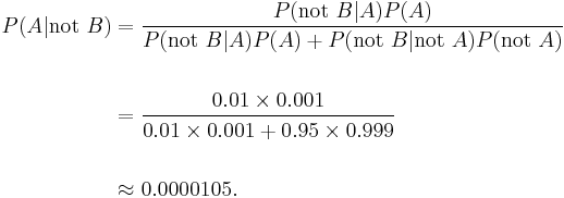
$\begin{align} P(A |\text{not }B) &= \frac{P(\text{not }B | A) P(A)}{P(\text{not }B | A)P(A) + P(\text{not }B |\text{not }A)P(\text{not }A)} \\ \\ &= \frac{0.01\times 0.001}{0.01 \times 0.001 + 0.95\times 0.999} \\ ~\\ &\approx 0.0000105.\end{align}$

The probability that a negative result is a false negative is about 0.0000105 or 0.00105%. When a disease is rare, false negatives will not be a major problem with the test.

But if 60% of the population had the disease, then the probability of a false negative would be greater. With the above test, the probability of a false negative would be

$\begin{align} P(A |\text{not }B) & = \frac{P(\text{not }B | A) P(A)}{P(\text{not }B | A)P(A) + P(\text{not }B |\text{not } A) P(\text{not }A)} \\ \\ &= \frac{0.01\times 0.6}{0.01 \times 0.6 + 0.95\times 0.4} \\ ~\\ &\approx 0.0155.\end{align}$

The probability that a negative result is a false negative rises to 0.0155 or 1.55%.

In the courtroom

Bayesian inference can be used in a court setting by an individual juror to coherently accumulate the evidence for and against the guilt of the defendant, and to see whether, in totality, it meets their personal threshold for 'beyond a reasonable doubt'.^[2]^[3]^[4]

Let $G$ denote the event that the defendant is guilty.

Let $E$ denote the event that the defendant's DNA matches DNA found at the crime scene.

Let $P(E|G)$ denote the probability of seeing event $E$ if the defendant is actually guilty. (Usually this would be taken to be near unity.)

Let $P(G|E)$ denote the probability that the defendant is guilty assuming the DNA match (event $E$ ).

Let $P(G)$ denote the juror's personal estimate of the probability that the defendant is guilty, based on the evidence other than the DNA match. This could be based on his responses under questioning, or previously presented evidence.

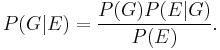
Bayesian inference tells us that if we can assign a probability p(G) to the defendant's guilt before we take the DNA evidence into account, then we can revise this probability to the conditional probability $P(G | E)$ , since

$P(G | E) = \frac{P(G) P(E | G)}{P(E)}.$

Suppose, on the basis of other evidence, a juror decides that there is a 30% chance that the defendant is guilty. Suppose also that the forensic testimony was that the probability that a person chosen at random would have DNA that matched that at the crime scene is 1 in a million, or 10⁻⁶.

The event E can occur in two ways. Either the defendant is guilty (with prior probability 0.3) and thus his DNA is present with probability 1, or he is innocent (with prior probability 0.7) and he is unlucky enough to be one of the 1 in a million matching people.

Thus the juror could coherently revise his opinion to take into account the DNA evidence as follows:

$P(G | E) = (0.3 \times 1.0) /(0.3 \times 1.0 + 0.7 \times 10^{-6}) = 0.99999766667.$

The benefit of adopting a Bayesian approach is that it gives the juror a formal mechanism for combining the evidence presented. The approach can be applied successively to all the pieces of evidence presented in court, with the posterior from one stage becoming the prior for the next.

The juror would still have to have a prior estimate for the guilt probability before the first piece of evidence is considered. It has been suggested that this could reasonably be the guilt probability of a random person taken from the qualifying population. Thus, for a crime known to have been committed by an adult male living in a town containing 50,000 adult males, the appropriate initial prior probability might be 1/50,000.

Adding up evidence.

For the purpose of explaining Bayes' theorem to jurors, it will usually be appropriate to give it in the form of betting odds rather than probabilities, as these are more widely understood. In this form Bayes' theorem states that

Posterior odds = prior odds x Bayes factor

In the example above, the juror who has a prior probability of 0.3 for the defendant being guilty would now express that in the form of odds of 3:7 in favour of the defendant being guilty, the Bayes factor is one million, and the resulting posterior odds are 3 million to 7 or about 429,000 to one in favour of guilt.

A logarithmic approach which replaces multiplication with addition and reduces the range of the numbers involved might be easier for a jury to handle. This approach, developed by Alan Turing during World War II and later promoted by I. J. Good and E. T. Jaynes among others, amounts to the use of information entropy.

In the United Kingdom, Bayes' theorem was explained to the jury in the odds form by a statistician expert witness in the rape case of Regina versus Denis John Adams. A conviction was secured but the case went to appeal, since no means of accumulating evidence had been provided for those jurors who did not wish to use Bayes' theorem. The Court of Appeal upheld the conviction, but it also gave their opinion that "To introduce Bayes' Theorem, or any similar method, into a criminal trial plunges the jury into inappropriate and unnecessary realms of theory and complexity, deflecting them from their proper task." No further appeal was allowed and the issue of Bayesian assessment of forensic DNA data remains controversial.

Gardner-Medwin^[5] argues that the criterion on which a verdict in a criminal trial should be based is not the probability of guilt, but rather the probability of the evidence, given that the defendant is innocent (akin to a frequentist p-value). He argues that if the posterior probability of guilt is to be computed by Bayes' theorem, the prior probability of guilt must be known. This will depend on the incidence of the crime, which is an unusual piece of evidence to consider in a criminal trial. Consider the following three propositions:

A: The known facts and testimony could have arisen if the defendant is guilty,

B: The known facts and testimony could have arisen if the defendant is innocent,

C: The defendant is guilty.

Gardner-Medwin argues that the jury should believe both A and not-B in order to convict. A and not-B implies the truth of C, but the reverse is not true. It is possible that B and C are both true, but in this case he argues that a jury should acquit, even though they know that they will be letting some guilty people go free. See also Lindley's paradox.

Other court cases in which probabilistic arguments played some role were the Howland will forgery trial, the Sally Clark case, and the Lucia de Berk case.

Search theory

In May 1968, the U.S. Navy's nuclear submarine USS Scorpion (SSN-589) failed to arrive as expected at her home port of Norfolk, Virginia. The command officers of the U.S. Navy were nearly convinced that the vessel had been lost off the Eastern Seaboard, but an extensive search there failed to discover the remains of the Scorpion.

Then, a Navy deep-water expert, John P. Craven, suggested that the USS Scorpion had sunk elsewhere. Craven organised a search southwest of the Azores based on a controversial approximate triangulation by hydrophones. He was allocated only a single ship, the Mizar, and he took advice from a firm of consultant mathematicians in order to maximise his resources. A Bayesian search methodology was adopted. Experienced submarine commanders were interviewed to construct hypotheses about what could have caused the loss of the Scorpion.

The sea area was divided up into grid squares and a probability assigned to each square, under each of the hypotheses, to give a number of probability grids, one for each hypothesis. These were then added together to produce an overall probability grid. The probability attached to each square was then the probability that the wreck was in that square. A second grid was constructed with probabilities that represented the probability of successfully finding the wreck if that square were to be searched and the wreck were to be actually there. This was a known function of water depth. The result of combining this grid with the previous grid is a grid which gives the probability of finding the wreck in each grid square of the sea if it were to be searched.

This sea grid was systematically searched in a manner which started with the high probability regions first and worked down to the low probability regions last. Each time a grid square was searched and found to be empty its probability was reassessed using Bayes' theorem. This then forced the probabilities of all the other grid squares to be reassessed (upwards), also by Bayes' theorem. The use of this approach was a major computational challenge for the time but it was eventually successful and the Scorpion was found about 740 kilometers southwest of the Azores in October of that year.

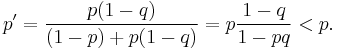
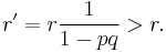
Suppose a grid square has a probability p of containing the wreck and that the probability of successfully detecting the wreck if it is there is q. If the square is searched and no wreck is found, then, by Bayes' theorem, the revised probability of the wreck being in the square is given by

$p' = \frac{p(1-q)}{(1-p)+p(1-q)} = p \frac{1-q}{1-pq} < p.$

For each other grid square, if its prior probability is r, its posterior probability is given by

$r' = r \frac{1}{1- pq} > r.$

Scientific method

The scientific method is sometimes interpreted as an application of Bayesian inference: In this view, Bayes' rule guides (or should guide) the updating of probabilities about hypotheses conditional on new observations or experiments.^[6]

Some experiments on belief revision have suggested that humans change their beliefs faster when using Bayesian methods than when using informal judgement.^[7] Bayesian methods have been used for hundreds of years, so there are many examples of Bayesian inference to scrutinize. Of the tens of thousands of papers published using Bayesian methods, few criticisms have been made of implausible priors in concrete applications. Such criticisms are themselves welcomed by Bayesian statisticians, as part of the inevitable revisions of science. For example, George E. P. Box and George C. Tiao said: "Inferences that are unacceptable must come from inappropriate assumption and not from inadequacies of the inferential system. Thus all parts of the model, including the prior distribution, are exposed to appropriate criticism."^[8] Nonetheless, worries about the possible problems of Bayesian methods continue to appear.^[9] Concern has been raised that a Bayesian view could be problematic for scientific judgements, since a Bayesian information processor (it is claimed) tends to confirm already established views and to suppress controversial views.^[10] Such worries have not so far been accompanied by experimental evidence that would challenge the perception that Bayesian methods facilitate belief revision, nor have examples been published of implausible priors whose use has led to practical problems in practical applications.

Relation to decision theory

A decision-theoretic justification of the use of Bayesian inference was given by Abraham Wald, who proved that every Bayesian procedure is admissible. Conversely, every admissible statistical procedure is either a Bayesian procedure or a limit of Bayesian procedures.^[11]

Wald's result also established the Bayesian approach as a fundamental technique in such areas of frequentist inference as point estimation, hypothesis testing, and confidence intervals. Wald characterized admissible procedures as Bayesian procedures (and limits of Bayesian procedures), making the Bayesian formalism a central technique in such areas of frequentist statistics as parameter estimation, hypothesis testing, and computing confidence intervals.^[12] For example:

"Under some conditions, all admissible procedures are either Bayes procedures or limits of Bayes procedures (in various senses). These remarkable results, at least in their original form, are due essentially to Wald. They are useful because the property of being Bayes is easier to analyze than admissibility."^[11]

"In decision theory, a quite general method for proving admissibility consists in exhibiting a procedure as a unique Bayes solution." ^[13]

"In the first chapters of this work, prior distributions with finite support and the corresponding Bayes procedures were used to establish some of the main theorems relating to the comparison of experiments. Bayes procedures with respect to more general prior distributions have played a very important in the development of statistics, including its asymptotic theory." "There are many problems where a glance at posterior distributions, for suitable priors, yields immediately interesting information. Also, this technique can hardly be avoided in sequential analysis."^[14]

"A useful fact is that any Bayes decision rule obtained by taking a proper prior over the whole parameter space must be admissible"^[15]
"An important area of investigation in the development of admissibility ideas has been that of conventional sampling-theory procedures, and many interesting results have been obtained." ^[16]

More mathematical examples

Naive Bayes classifier

See naive Bayes classifier.

Posterior distribution of the binomial parameter

In this example we consider the computation of the posterior distribution for the binomial parameter. This is the same problem considered by Bayes in Proposition 9 of his essay.

We are given m observed successes and n observed failures in a binomial experiment. The experiment may be tossing a coin, drawing a ball from an urn, or asking someone their opinion, among many other possibilities. What we know about the parameter (let's call it a) is stated as the prior distribution, p(a).

For a given value of a, the probability of m successes in m + n trials is

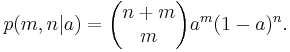
$p(m,n|a) = \begin{pmatrix} n+m \\ m \end{pmatrix} a^m (1-a)^n.$

Since m and n are fixed, and a is unknown, this is a likelihood function for a. From the continuous form of the law of total probability we have

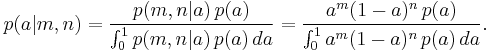
$p(a|m,n) = \frac{p(m,n|a)\,p(a)}{\int_0^1 p(m,n|a)\,p(a)\,da} = \frac{a^m (1-a)^n\,p(a)} {\int_0^1 a^m (1-a)^n\,p(a)\,da}.$

For some special choices of the prior distribution p(a), the integral can be solved and the posterior takes a convenient form. In particular, if p(a) is a beta distribution with parameters m₀ and n₀, then the posterior is also a beta distribution with parameters m + m₀ and n + n₀.

A conjugate prior is a prior distribution, such as the beta distribution in the above example, which has the property that the posterior is the same type of distribution.

What is "Bayesian" about Proposition 9 is that Bayes presented it as a probability for the parameter a. That is, not only can one compute probabilities for experimental outcomes, but also for the parameter which governs them, and the same algebra is used to make inferences of either kind. Interestingly, Bayes actually states his question in a way that might make the idea of assigning a probability distribution to a parameter palatable to a frequentist. He supposes that a billiard ball is thrown at random onto a billiard table, and that the probabilities p and q are the probabilities that subsequent billiard balls will fall above or below the first ball. By making the binomial parameter a depend on a random event, he cleverly escapes a philosophical quagmire that was an issue he most likely was not even aware of.

Computer applications

Bayesian inference has applications in artificial intelligence and expert systems. Bayesian inference techniques have been a fundamental part of computerized pattern recognition techniques since the late 1950s. There is also an ever growing connection between Bayesian methods and simulation-based Monte Carlo techniques since complex models cannot be processed in closed form by a Bayesian analysis, while a graphical model structure may allow for efficient simulation algorithms like the Gibbs sampling and other Metropolis-Hastings algorithm schemes. Recently Bayesian inference has gained popularity amongst the phylogenetics community for these reasons; a number of applications allow many demographic and evolutionary parameters to be estimated simultaneously. In the areas of population genetics and dynamical systems theory approximate Bayesian computation (ABC) are also becoming increasingly popular.

As applied to statistical classification, Bayesian inference has been used in recent years to develop algorithms for identifying e-mail spam. Applications which make use of Bayesian inference for spam filtering include DSPAM, Bogofilter, SpamAssassin, SpamBayes, and Mozilla. Spam classification is treated in more detail in the article on the naive Bayes classifier.

In some applications fuzzy logic is an alternative to Bayesian inference. Fuzzy logic and Bayesian inference, however, are mathematically and semantically not compatible. You cannot, in general, understand the degree of truth in fuzzy logic as probability and vice versa; fuzziness measures "the degree to which an event occurs, not whether it occurs"^[17].

History

The term Bayesian refers to Thomas Bayes (1702–1761), who proved a special case of what is now called Bayes' theorem. However, it was Pierre-Simon Laplace (1749–1827) who introduced a general version of the theorem and used it to approach problems in celestial mechanics, medical statistics, reliability, and jurisprudence ^[18]. Early Bayesian inference, which used uniform priors following Laplace's principle of insufficient reason, was called "inverse probability" (because it infers backwards from observations to parameters, or from effects to causes^[19]). After the 1920s, "inverse probability" was largely supplanted by a collection of methods that came to be called frequentist statistics.^[19]

In the 20th century, the ideas of Laplace were further developed in two different directions, giving rise to objective and subjective currents in Bayesian practice. In the objectivist stream, the statistical analysis depends on only the model assumed and the data analysed.^[20]. No subjective decisions need to be involved. In contrast, "subjectivist" statisticians deny the possibility of fully objective analysis for the general case.

In the 1980s, there was a dramatic growth in research and applications of Bayesian methods, mostly attributed to the discovery of Markov chain Monte Carlo methods, which removed many of the computational problems, and an increasing interest in nonstandard, complex applications.^[21] Despite growth of Bayesian research, most undergraduate teaching is still based on frequentist statistics.^[22] Nonetheless, Bayesian methods are widely accepted and used, such as for example in the field of machine learning.^[23]

Notes

↑ Douglas Hubbard "How to Measure Anything: Finding the Value of Intangibles in Business" pg. 46, John Wiley & Sons, 2007
↑ Dawid, A.P. and Mortera, J. (1996) "Coherent analysis of forensic identification evidence". Journal of the Royal Statistical Society, Series B, 58,425–443.
↑ Foreman, L.A; Smith, A.F.M. and Evett, I.W. (1997). "Bayesian analysis of deoxyribonucleic acid profiling data in forensic identification applications (with discussion)". Journal of the Royal Statistical Society, Series A, 160, 429-469.
↑ Robertson, B. and Vignaux, G.A. (1995) Interpreting Evidence: Evaluating Forensic Science in the Courtroom. John Wiley and Sons. Chichester. ISBN 978-0-471-96026-3
↑ Gardner-Medwin, A. (2005) "What probability should the jury address?". Significance, 2 (1), March 2005
↑ Howson & Urbach (2005), Jaynes (2003)
↑ Edwards (1968,1982), Phillips & Edwards (2008)
↑ Box & Tiao (1973,page 9, point 4)
↑ Clark Glymour (1980), "Why I Am Not a Bayesian", Theory and Evidence, Princeton Univ Press, ISBN 069107240X (Chapter III)
↑ Jonathan J. Koehler. (1993). "The influence of prior beliefs on scientific judgments of evidence quality". Organizational Behavior and Human Decision Processes. 56, 28–55.
↑ ^11.0 ^11.1 Bickel & Doksum (2001, page 32)
↑ * Kiefer, J. and Schwartz, R. (1965). "Admissible Bayes character of T²-, R²-, and other fully invariant tests for multivariate normal problems". Annals of Mathematical Statistics 36: pp. 747–770.
- Schwartz, R. (1969). "Invariant proper Bayes tests for exponential families". Annals of Mathematical Statistics 40: pp. 270–283.
- Hwang, J. T. and Casella, George (1982). "Minimax confidence sets for the mean of a multivariate normal distribution". Annals of Statistics 10: pp. 868–881.
↑ Lehmann, Erich (1986). Testing Statistical Hypotheses (Second ed.). (see page 309 of Chapter 6.7 "Admissibilty", and pages 17–18 of Chapter 1.8 "Complete Classes"
↑ Le Cam, Lucien (1986). Asymptotic Methods in Statistical Decision Theory. Springer-Verlag. (From "Chapter 12 Posterior Distributions and Bayes Solutions", page 324)
↑ Cox, D. R. and Hinkley, D. V (1974). Theoretical Statistics. Chapman and Hall. page 432
↑ Cox, D. R. and Hinkley, D. V (1974). Theoretical Statistics. Chapman and Hall. page 433)
↑ Kosko, Bart (1992). Neural Networks and Fuzzy Systems: a dynamical systems approach to machine intelligence (1st ed.). Englewood Cliffs, NJ, USA.: Prentice Hall. p. 265. ISBN 9780136114352.
↑ Stephen M. Stigler (1986) The history of statistics. Harvard University press. Chapter 3.
↑ ^19.0 ^19.1 Stephen. E. Fienberg, (2006) "When did Bayesian Inference become "Bayesian"? Bayesian Analysis, 1 (1), 1–40. See page 5.
↑ JM. Bernardo (2005), "Reference analysis", Handbook of statistics, 25, 17–90
↑ Wolpert, RL. (2004) A conversation with James O. Berger, Statistical science, 9, 205–218
↑ José M. Bernardo (2006) A Bayesian mathematical statistics prior. ICOTS-7
↑ Bishop, C.M. (2007) Pattern Recognition and Machine Learning. Springer, 2007

References

Bickel, Peter J. and Doksum, Kjell A. (2001). Mathematical Statistics, Volume 1: Basic and Selected Topics (Second (updated printing 2007) ed.). Pearson Prentice–Hall. ISBN 013850363X.
Box, G.E.P. and Tiao, G.C. (1973) Bayesian Inference in Statistical Analysis, Wiley, ISBN 0-471-57428-7
Edwards, Ward (1968). "Conservatism in Human Information Processing". In Kleinmuntz, B. Formal Representation of Human Judgment. Wiley.
Edwards, Ward (1982). "Conservatism in Human Information Processing (excerpted)". In Daniel Kahneman, Paul Slovic and Amos Tversky. Judgment under uncertainty: Heuristics and biases. Cambridge University Press.
Jaynes E.T. (2003) Probability Theory: The Logic of Science, CUP. ISBN 9780521592710 (Link to Fragmentary Edition of March 1996).
Howson, C. and Urbach, P. (2005). Scientific Reasoning: the Bayesian Approach (3rd ed.). Open Court Publishing Company. ISBN 978-0812695786.
Phillips, L.D.; Edwards, W. (October 2008). "Chapter 6: Conservatism in a simple probability inference task (Journal of Experimental Psychology (1966) 72: 346-354)". In Jie W. Weiss and David J. Weiss. A Science of Decision Making:The Legacy of Ward Edwards. Oxford University Press. pp. 536. ISBN 9780195322989.

External links

Bayesian Statistics summary from Scholarpedia.
A nice on-line introductory tutorial to Bayesian probability from Queen Mary University of London
An Intuitive Explanation of Bayesian Reasoning Bayes' Theorem for the curious and bewildered; an excruciatingly gentle introduction by Eliezer Yudkowsky
Paul Graham. "A Plan for Spam" (exposition of a popular approach for spam classification)
Commentary on Regina versus Adams
Mathematical notes on Bayesian statistics and Markov chain Monte Carlo
Bayesian Rating/Ranking How to implement Bayes' Theorem for online rating and ranking systems
Bayesian reading list, categorized and annotated. Designed for cognitive science; maintained by Tom Griffiths.
Stanford Encyclopedia of Philosophy: Inductive Logic a comprehensive Bayesian treatment of Inductive Logic and Confirmation Theory
Confirmation Theory An extensive presentation of Bayesian Confirmation Theory
What is Bayesian Learning?

Statistics

Descriptive statistics

Continuous data

Location	Mean (Arithmetic, Geometric, Harmonic) · Median · Mode

Dispersion	Range · Standard deviation · Coefficient of variation · Percentile · Interquartile range

Shape	Variance · Skewness · Kurtosis · Moments · L-moments

Count data

Index of dispersion

Summary tables

Grouped data · Frequency distribution · Contingency table

Dependence

Pearson product-moment correlation · Rank correlation (Spearman's rho, Kendall's tau) · Partial correlation · Scatter plot

Statistical graphics

Bar chart · Biplot · Box plot · Control chart · Correlogram · Forest plot · Histogram · Q-Q plot · Run chart · Scatter plot · Stemplot · Radar chart

Data collection

Designing studies	Effect size · Standard error · Statistical power · Sample size determination

Survey methodology	Sampling · Stratified sampling · Opinion poll · Questionnaire

Controlled experiment	Design of experiments · Randomized experiment · Random assignment · Replication · Blocking · Regression discontinuity · Optimal design

Uncontrolled studies	Natural experiment · Quasi-experiment · Observational study

Statistical inference

Bayesian inference	Bayesian probability · Prior · Posterior · Credible interval · Bayes factor · Bayesian estimator · Maximum posterior estimator

Frequentist inference	Confidence interval · Hypothesis testing · Sampling distribution · Meta-analysis

Specific tests	Z-test (normal) · Student's t-test · F-test · Chi-square test · Pearson's chi-square · Wald test · Mann–Whitney U · Shapiro–Wilk · Signed-rank · Likelihood-ratio

General estimation	Mean-unbiased · Median-unbiased · Maximum likelihood · Method of moments · Minimum distance · Maximum spacing · Density estimation

Correlation and regression analysis

Correlation	Pearson product-moment correlation · Partial correlation · Confounding variable · Coefficient of determination

Regression analysis	Errors and residuals · Regression model validation · Mixed effects models · Simultaneous equations models

Linear regression	Simple linear regression · Ordinary least squares · General linear model · Bayesian regression

Non-standard predictors	Nonlinear regression · Nonparametric · Semiparametric · Isotonic · Robust

Generalized linear model	Exponential families · Logistic (Bernoulli) · Binomial · Poisson

Formal analyses	Analysis of variance (ANOVA) · Analysis of covariance · Multivariate ANOVA

Data analyses and models for other specific data types


Multivariate statistics	Multivariate regression · Principal components · Factor analysis · Cluster analysis · Copulas

Time series analysis	Decomposition · Trend estimation · Box–Jenkins · ARMA models · Spectral density estimation

Survival analysis	Survival function · Kaplan–Meier · Logrank test · Failure rate · Proportional hazards models · Accelerated failure time model

Categorical data	McNemar's test · Cohen's kappa

Applications

Engineering statistics	Methods engineering · Probabilistic design · Process & Quality control · Reliability · System identification

Environmental statistics	Geostatistics · Climatology

Medical statistics	Epidemiology · Clinical trial · Clinical study design

Social statistics	Actuarial science · Population · Demography · Census · Psychometrics · Official statistics · Crime statistics

Category · Portal · Outline · Index